You may have read about how to find the magnetic field from a very long wire of current. Now, what is the magnetic field from a single segment? Suppose we have the configuration shown below. Your observation point is at the origin, and the segment of current $I$ runs in a straight line from $\langle -L, 0, 0 \rangle$ to $\langle 0, -L, 0 \rangle$.

• The current in the segment is $I$.
• The observation point is at the origin.
• The segment stretches from from $\langle -L, 0, 0 \rangle$ to $\langle 0, -L, 0 \rangle$.

• $\vec{B}$

• The current is steady, and the wire segment is uniform.

• We represent the Biot-Savart Law for magnetic field from a current as

$$\vec{B}= \int \frac{\mu_0}{4 \pi}\frac{I \cdot d\vec{l}\times \vec{r}}{r^3}$$

• We represent the situation with diagram given above.

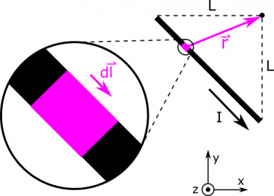
Below, we show a diagram with a lot of pieces of the Biot-Savart Law unpacked. We show an example $\text{d}\vec{l}$, and a separation vector $\vec{r}$. Notice that $\text{d}\vec{l}$ is directed along the segment, in the same direction as the current. The separation vector $\vec{r}$ points as always from source to observation.

For now, we write

$$\text{d}\vec{l} = \langle \text{d}x, \text{d}y, 0 \rangle$$ and $$\vec{r} = \vec{r}_{obs} - \vec{r}_{source} = 0 - \langle x, y, 0 \rangle = \langle -x, -y, 0 \rangle$$ Notice that we can rewrite $y$ as $y=-L-x$. This is a little tricky to arrive at, but is necessary to figure out unless you rotate your coordinate axes, which would be an alternative solution to this example. If finding $y$ is troublesome, it may be helpful to rotate. We can take the derivative of both sides to find $\text{d}y=-\text{d}x$. We can now plug in to express $\text{d}\vec{l}$ and $\vec{r}$ in terms of $x$ and $\text{d}x$: $$\text{d}\vec{l} = \langle \text{d}x, -\text{d}x, 0 \rangle$$ $$\vec{r} = \langle -x, L+x, 0 \rangle$$ Now, a couple other quantities that we see will be useful: $$\text{d}\vec{l} \times \vec{r} = \langle 0, 0, \text{d}x(L+x) - (-\text{d}x)(-x) \rangle = \langle 0, 0, L\text{d}x \rangle = L\text{d}x \hat{z}$$ $$r^3 = (x^2 + (L+x)^2)^{3/2}$$ The last thing we need is the bounds on our integral. Our variable of integration is $x$, since we chose to express everything in terms of $x$ and $\text{d}x$. Our segment begins at $x=-L$, and ends at $x=0$, so these will be the limits on our integral. Below, we write the integral all set up, and then we evaluate using some assistance some Wolfram Alpha. $$\begin{align*} \vec{B} &= \int \frac{\mu_0}{4 \pi}\frac{I \cdot d\vec{l}\times \vec{r}}{r^3} \\ &= \int_{-L}^0 \frac{\mu_0}{4 \pi}\frac{IL\text{d}x}{(x^2 + (L+x)^2)^{3/2}}\hat{z} \\ &= \frac{\mu_0}{2 \pi}\frac{I}{L}\hat{z} \end{align*}$$