In these notes, we will examine a few examples of changing magnetic fluxes and associated induced voltages. Recall from the previous notes that these are related by Faraday's Law which says:

$$V_{ind} = -\frac{d\Phi_b}{dt}$$

This is saying that the induced current is the negative slope of the magnetic flux. In other words, if the magnetic flux is increasing, then $V_{ind}$ will be negative, if the magnetic flux is decreasing, then $V_{ind}$ will be positive, and if the magnetic flux is constant, then $V_{ind} = 0$.

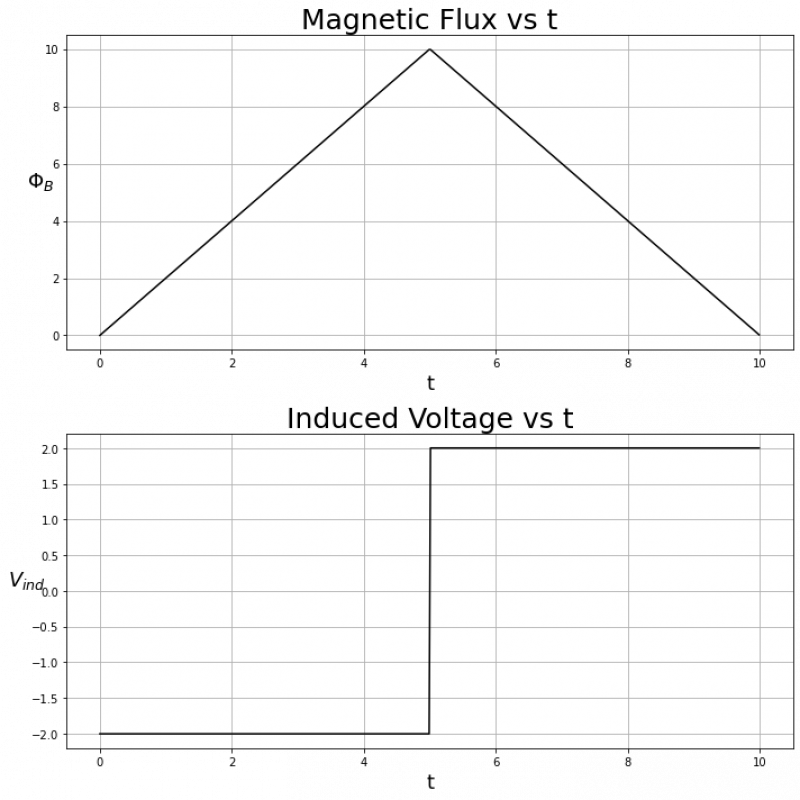
First let's consider when an example where $\Phi_B$ rises and falls linearly with the same magnitude of slope:

From $t = 0$ to $t = 5$, $\Phi_B(t)$ has a constant positive slope, so $V_{ind}$ will be constant and negative. Conversely, from $t = 5$ to $t = 10$, $\Phi_B(t)$ has a constant negative slope, so $V_{ind}$ will be constant and positive.

Specifically, in this case $\Phi_B(t)$ is defined as: $$ \Phi_B(t)= \begin{cases} 2t & \text{if } 0<t<5\\ -2t & \text{if } 5<t<10 \end{cases} $$ Which means $\frac{d \Phi_B}{dt}$ is: $$ \frac{d \Phi_B}{dt}= \begin{cases} 2 & \text{if } 0<t<5\\ -2 & \text{if } 5<t<10 \end{cases} $$ Now we can multiply by $-1$ because of the negative sign in Faraday's law to find $V_{ind}$: $$ V_{ind}= \begin{cases} -2 & \text{if } 0<t<5\\ 2 & \text{if } 5<t<10 \end{cases} $$

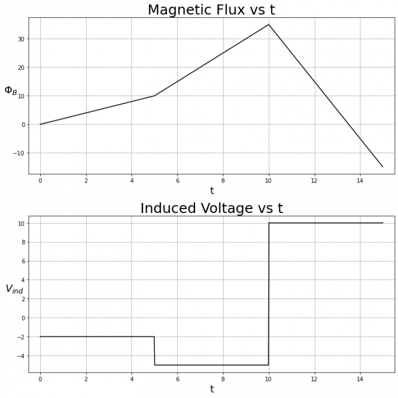
Next, let's consider an example with a few different slopes:

We can see that from $t=0$ to $t = 10$, $\Phi_B(t)$ has a positive slope, so $V_{ind}$ is negative on that time interval. However, $\Phi_B(t)$ is steeper from $t=5$ to $t=10$, so $V_{ind}$ is more negative on that time interval than from $t = 0$ to $t = 5$. From $t = 10$ to $t = 15$, $\Phi_B(t)$ has a constant and negative slope, so $V_{ind}$ is constant and positive on that time interval. Specifically we have that:

$$ \Phi_B(t)= \begin{cases} 2t & \text{if } 0<t<5\\ 5t -15 & \text{if } 5<t<10\\ -10t + 135 & \text{if } 10<t<15 \end{cases} $$ Which means $\frac{d \Phi_B}{dt}$ is: $$ \frac{d \Phi_B}{dt}= \begin{cases} 2 & \text{if } 0<t<5\\ 5 & \text{if } 5<t<10\\ -10 & \text{if } 10<t<15 \end{cases} $$ Which finally means that $V_{ind}$ is: $$ V_{ind}= \begin{cases} -2 & \text{if } 0<t<5\\ -5 & \text{if } 5<t<10\\ 10 & \text{if } 10<t<15 \end{cases} $$

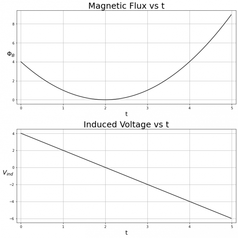
Finally, let's look at an example with a non-linear $\Phi_B(t)$:

$\Phi_B(t)$ looks like a quadratic centered about t = 2. We can see that while $\Phi_B(t)$ is decreasing ($0<t<2$), $V_{ind}$ is positive, and while $\Phi_B(t)$ is increasing ($2<t<8$), $V_{ind}$ is negative.

Specifically, in this case we have:

$$\Phi_B(t) = (t-2)^2$$

Taking a first derivative with respect to time yields:

$$\frac{d \Phi_B}{dt} = 2(t-2)$$

Multiplying by $-1$ to find $V_{ind}$ gives:

$$V_{ind} = -2(t-2)$$