Suppose we have a segment of uniformly distributed charge stretching from the point $\langle 0,0,0 \rangle$ to $\langle 1 \text{ m}, 1 \text{ m}, 0 \rangle$, which has total charge $Q$. We also have a point $P=\langle 2 \text{ m},0,0 \rangle$. Define a convenient $\text{d}Q$ for the segment, and $\vec{r}$ between a point on the segment to the point $P$. Also, give appropriate limits on an integration over $\text{d}Q$ (you don't have to write any integrals, just give appropriate start and end points). First, do this for the given coordinate axes. Second, define a new set of coordinate axes to represent $\text{d}Q$ and $\vec{r}$ in a simpler way and redo.

• The segment stretches from $\langle 0,0,0 \rangle$ to $\langle 1 \text{ m}, 1 \text{ m}, 0 \rangle$.
• The segment has a charge $Q$, which is uniformly distributed.
• $P=\langle 2 \text{ m},0,0 \rangle$.

• $\text{d}Q$ and $\vec{r}$
• A new set of coordinate axes

• The thickness of the segment is infinitesimally small, and we can approximate it as a line segment.
• The total charge is a constant - not discharging.

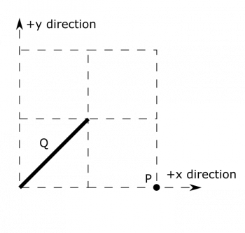
• For the first part, we can draw a set of coordinate axes using what we already know. The first part of the example involves the following orientation:

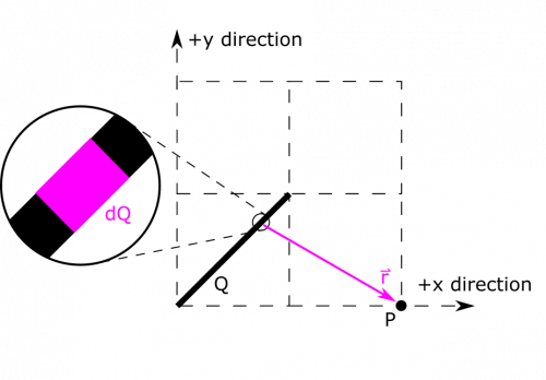
• We can represent $\text{d}Q$ and $\vec{r}$ for our line as follows:

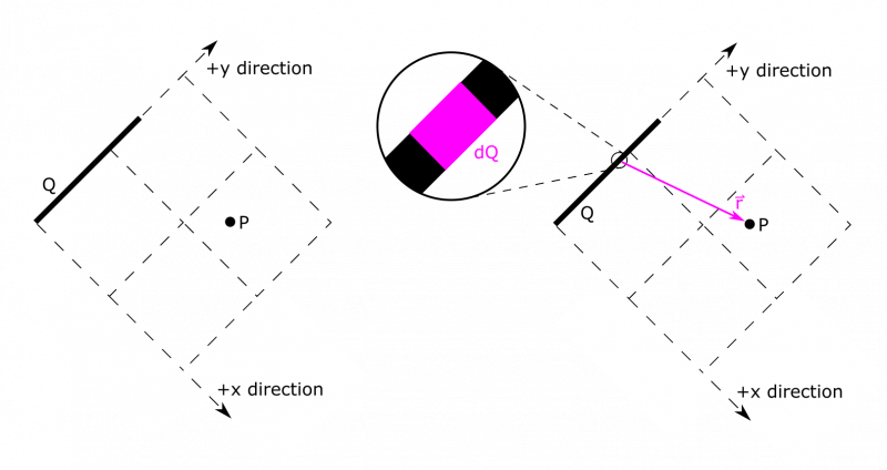
• For the second part when we define a new set of coordinate axes, it makes sense to line up the segment along an axis. We choose the $y$-axis. We could have chosen the $x$-axis, and arrived at a very similar answer. Whichever you like is fine!

Some note about picking dx instead of dy is completely arbitrary

In the first set of axes, the segment extends in the $x$ and $y$ directions. A simple calculation of the Pythagorean theorem tells us the total length of the segment is $\sqrt{2}$, so we can define the line charge density $\lambda=Q/\sqrt{2}$. When we define $\text{d}l$, we want it align with the segment, so we can have $\text{d}l=\sqrt{\text{d}x^2+\text{d}y^2}$. Since $x=y$ along the segment, we can simplify a little bit. $\text{d}l=\sqrt{\text{d}x^2+\text{d}x^2}=\sqrt{2}\text{d}x$. Now, we can write an expression for $\text{d}Q$: $$\text{d}Q=\lambda\text{d}l=\frac{\sqrt{2}}{\sqrt{2}}Q\text{d}x=Q\text{d}x$$ This is a little funky - the units look weird here because one of $\sqrt{2}$'s that cancelled out had units and one did not. It might make sense to try to track the units more closely.

The units here might look a little weird, since distance was defined without dimensions in the example statement. Next, we need $\vec{r}$. We will put it in terms of $x$, not $y$, just as we did for $\text{d}Q$. (Note that while the initial variable picking was arbitrary we now have to match) We know $\vec{r}_P=\langle 2,0,0 \rangle$, and $\vec{r}_{\text{d}Q}=\langle x, y, 0 \rangle$. Again, $x=y$, so we can rewrite $\vec{r}_{\text{d}Q}=\langle x, x, 0 \rangle$. We now have enough to write $\vec{r}$: $$\vec{r}=\vec{r}_P-\vec{r}_{\text{d}Q}=\langle 2-x, -x, 0 \rangle$$ Because we picked dx and x as our variable, we are all set up to integrate over $x$. This means that our limits of integration also have to match the total length that we want to add up in terms of the x variable, which goes from $0$ to $1$. So our limits of integration would be from $0$ to $1$.

In the second set of axes, the segment extends only in the $y$ direction. This problem is now very similar to the examples in the notes. The length of the segment is still $\sqrt{2}$, so we can define the line charge density $\lambda=Q/\sqrt{2}$. When we define $\text{d}l$, we want it align with the segment, which is much simpler this time: $\text{d}l=\text{d}y$. Now, we can write an expression for $\text{d}Q$: $$\text{d}Q=\lambda\text{d}l=\frac{Q\text{d}y}{\sqrt{2}}$$ Next, we need $\vec{r}$. We will put it in terms of $y$, just as we did for $\text{d}Q$. The location of $P$ is a little different with this new set of axes. Now, we have $\vec{r}_P=\langle \sqrt{2},\sqrt{2},0 \rangle$, and $\vec{r}_{\text{d}Q}=\langle 0, y, 0 \rangle$. We have enough to write $\vec{r}$: $$\vec{r}=\vec{r}_P-\vec{r}_{\text{d}Q}=\langle \sqrt{2}, \sqrt{2}-y, 0 \rangle$$ (Match similar wording to that above.) An integration would occur over $y$, which goes from $0$ to $\sqrt{2}$. These would be our limits of integration.