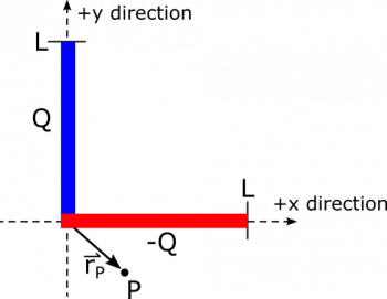
Suppose we have two segments of uniformly distributed charge, one with total charge $+Q$, the other with $-Q$. The two segments each have length $L$, and lie crossed at their endpoints in the $xy$-plane. The segment with charge $+Q$ lies along the $y$-axis, and the segment with charge $-Q$ lies along the $x$-axis. See below for a diagram of the situation. Create an expression for the electric field $\vec{E}_P$ at a point $P$ that is located at $\vec{r}_P=r_x\hat{x}+r_y\hat{y}$. You don't have to evaluate integrals in the expression.

• One segment lies on the $y$-axis stretching from $0$ to $L$, with charge $Q$ uniformly distributed.
• The other segment lies on the $x$-axis stretching from $0$ to $L$, with charge $-Q$ uniformly distributed.
• The point $P$ is at the arbitrary location $\vec{r}_P=r_x\hat{x}+r_y\hat{y}$
• The electric field due to a point charge is $$\vec{E} = \frac{1}{4\pi\epsilon_0}\frac{q}{r^3}\vec{r}$$
• The electric field at $P$ is the superposition of contributions from the two segments: $$\vec{E}_P = \vec{E}_{+Q} +\vec{E}_{-Q}$$

• Find $\vec{E}_P$.

• The thicknesses of both segments are infinitesimally small, and we can approximate them as line segments.

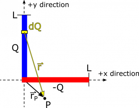
Because we know that electric fields add through superposition, we can treat of the charges separately, find the electric field, then add the fields together at $P$ at the end. We can begin with the electric field due to the segment along the $y$-axis. We start by finding $\text{d}Q$ and $\vec{r}$. The charge is uniformly distributed so we have a simple line charge density of $\lambda=Q/L$. The segment extends in the $y$-direction, so we have $\text{d}l=\text{d}y$. This gives us $\text{d}Q$: $$\text{d}Q=\lambda\text{d}l=\frac{Q\text{d}y}{L}$$

The separation vector $\vec{r}$ points from the source of the electric field to the observation point. The source is $\text{d}Q$, which is located at $y\hat{y}$, and the observation point is $\vec{r}_P=r_x\hat{x}+r_y\hat{y}$. Then we have the separation vector: $$\vec{r}=\vec{r}_P-y\hat{y}=r_x\hat{x}+r_y\hat{y}-y\hat{y}=r_x\hat{x}+(r_y-y)\hat{y}$$

Now, we have enough to define the electric field from the small piece ($\text{d}Q$) of the segment - plugging the $\text{d}Q$ and $\vec{r}$ we just found: $$\text{d}\vec{E}=\frac{1}{4\pi\epsilon_0}\frac{\text{d}Q}{r^3}\vec{r}=\frac{1}{4\pi\epsilon_0}\frac{Q\text{d}y}{L\cdot|r_x\hat{x}+(r_y-y)\hat{y}|^3}(r_x\hat{x}+(r_y-y)\hat{y})$$

Next, we integrate over the entire segment to find an expression for its contribution to the electric field vector at $P$. The limits of our integral are based on the variable of integration, which is $y$. This denotes the length along the segment on the $y$-axis, which stretches from $0$ to $L$, so these are our limits of integration. $$\vec{E}_{+Q}=\int_0^L\frac{1}{4\pi\epsilon_0}\frac{Q\text{d}y}{L\cdot|r_x\hat{x}+(r_y-y)\hat{y}|^3}(r_x\hat{x}+(r_y-y)\hat{y})$$

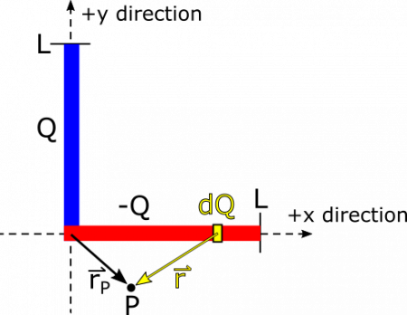
Next, we can do a similar analysis to find the electric field vector contribution from the segment that lies along the $x$-axis. See below for a visual of $\text{d}Q$ and $\vec{r}$. See if you can convince yourself that for the segment along the $x$-axis, $\text{d}Q=\frac{-Q\text{d}x}{L}$, and $\vec{r}=(r_x-x)\hat{x}+r_y\hat{y}$.

From here, we can find $\text{d}\vec{E}$: $$\text{d}\vec{E}=\frac{1}{4\pi\epsilon_0}\frac{\text{d}Q}{r^3}\vec{r}=\frac{1}{4\pi\epsilon_0}\frac{-Q\text{d}x}{L\cdot|(r_x-x)\hat{x}+r_y\hat{y}|^3}((r_x-x)\hat{x}+r_y\hat{y})$$

To find the contribution from the entire segment, we again must determine the endpoints of our integration. Our variable of integration is $x$ this time, which denotes the distance along the segment that lies on the $x$-axis. This distance stretches from $0$ to $L$, so these are our limits of integration: $$\vec{E}_{-Q}=\int_0^L\frac{1}{4\pi\epsilon_0}\frac{-Q\text{d}x}{L\cdot|(r_x-x)\hat{x}+r_y\hat{y}|^3}((r_x-x)\hat{x}+r_y\hat{y})$$

Then the final electric field vector at $P$ is the sum of the two contributions, because of vector superposition. (You can pull out the constants to simplify the integral if you want.) \begin{align*} \vec{E} &= \vec{E}_{+Q}+\vec{E}_{-Q} \\ &= \int_0^L\frac{1}{4\pi\epsilon_0}\frac{Q\text{d}y}{L\cdot|r_x\hat{x}+(r_y-y)\hat{y}|^3}(r_x\hat{x}+(r_y-y)\hat{y}) + \int_0^L\frac{1}{4\pi\epsilon_0}\frac{-Q\text{d}x}{L\cdot|(r_x-x)\hat{x}+r_y\hat{y}|^3}((r_x-x)\hat{x}+r_y\hat{y}) \\ &= \frac{Q}{4\pi\epsilon_0L}\left(\int_0^L\frac{\text{d}y}{|r_x\hat{x}+(r_y-y)\hat{y}|^3}(r_x\hat{x}+(r_y-y)\hat{y}) - \int_0^L\frac{\text{d}x}{|(r_x-x)\hat{x}+r_y\hat{y}|^3}((r_x-x)\hat{x}+r_y\hat{y})\right) \\ \end{align*} At this point we have the integrals set up, which you could solve by hand if you so desire or plug them into Wolfram Alpha, Mathematica, or some other computation program.